Deep Hierarchical Unsupervised Intent Modelling: Getting Value Without Training Data

Businesses run on communication - customers reach out when they want something, colleagues communicate to get work done. Every message counts. Our mission at Re:infer is to unlock the value in these messages and to help every team in a business deliver better products and services efficiently and at scale.

With that goal, we continuously research and develop our core machine learning and natural language understanding technology. The machine learning models at Re:infer use pre-training, unsupervised learning, semi-supervised learning and active learning to deliver state of the art accuracy with minimal time and investment from our users.

In this research post, we explore a new unsupervised approach to automatically recognising the topics and intents, and their taxonomy structure, from a communications dataset. It's about improving the quality of the insights we deliver and the speed with which these are obtained.

Abstract

Topic models are a class of methods for discovering the "topics" that occur in a collection of "documents". Importantly, topic models work without having to collect any labelled training data. They automatically identify the topics in a dataset and which topics appear in each document.

A hypothetical "failing trade" email and the types of hierarchical topics we'd like to automatically infer.

In this post:

• We explain traditional topic models and discuss some of their weaknesses, e.g. that the number of topics must be known in advance, the relationships between topics are not captured, etc.
• We organise the topics into a hierarchy which is automatically inferred based on the dataset’s topical structure. The hierarchy groups together semantically related topics.
• We achieve a more coherent topic hierarchy by incorporating Transformer-based embeddings into the model.

Background

Topic models assume that a dataset (collection of documents) contains a set of topics. A topic specifies how likely each word is to occur in a document. Each document in the dataset is generated from a mixture of the topics. Generally, sets of words which frequently occur together will have high probability in a given topic.

For example, suppose we have a dataset made up of the following documents:

• Document 1: "dogs are domesticated descendants of wolves"
• Document 2: "cats are carnivorous mammals with whiskers and retractable claws"
• Document 3: "big cats have been known to attack dogs"
• Document 4: "after being scratched by the sharp claws of cats, some dogs can become fearful of cats"
• Document 5: "domesticated dogs may prefer the presence of cats to other dogs"

A topic model trained on these documents may learn the following topics and document-topic assignments:

Topic 1	Topic 2
dogs	cats
domesticated	claws
wolves	whiskers
...	...

Example topics with words sorted by highest probability.

	Topic 1	Topic 2
Document 1	100%	0%
Document 2	0%	100%
Document 3	50%	50%
Document 4	33%	67%
Document 5	67%	33%

Example document-topic assignments.

Viewing the most likely words for each topic, as well as which topics each document belongs to, provides an overview of what the text in a dataset is about and which documents are similar to each other.

Embedded Topic Models

The canonical topic model is called Latent Dirichlet Allocation (LDA). It is a generative model, trained using (approximate) maximum likelihood estimation. LDA assumes that:

• There are $K$ topics, each of which specifies a distribution over the vocabulary (the set of words in the dataset).
• Each document (collection of words) has a distribution over topics.
  • Each word in a document is generated from one topic, according to the document’s distribution over topics and the topic’s distribution over the vocabulary.

Most modern topic models are built on LDA; initially we focus on the Embedded Topic Model (ETM). The ETM uses embeddings to represent both words and topics. In traditional topic modelling, each topic is a full distribution over the vocabulary. In the ETM however, each topic is a vector in the embedding space. For each topic, the ETM uses the topic embedding to form a distribution over the vocabulary.

Training and Inference

The generative process for a document is as follows:

1. Sample the latent representation $\mathbf{z}$ from the prior distribution: $\mathbf{z} \sim \mathcal{N}(\mathbf{0}, \mathbf{I})$.
2. Compute the topic proportions $\pmb{\theta} = \operatorname{softmax}(\mathbf{z})$.
3. For each word $w$ in the document:
   1. Sample the latent topic assignment $y_{w} \sim \operatorname{Cat}(\pmb{\theta})$.
   2. Sample the word $x_{w} \sim \operatorname{Cat}(\operatorname{softmax}(\mathbf{U} \cdot \mathbf{t}_{y_{w}}))$.

where $\mathbf{U} \in \mathbb{R}^{V \times E}$ is the word embedding matrix and $\mathbf{t}_{y_{w}} \in \mathbb{R}^{E}$ is the embedding of topic $y_{w}$; these are the model parameters. $V$ is the number of words in the vocabulary and $E$ is the embedding size.

The log-likelihood for a document with words $v_{1}, v_{2}, \dots, v_{w}$ is:

$$\log p(x_{1}=v_{1}, \dots, x_{W}=v_{W}) = \log \int_{\mathbf{z}} p(\mathbf{z}) \prod_{w=1}^{W} p(x_{w}=v_{w}|\mathbf{z})$$

where:

$$p(x_{w}=v_{w}|\mathbf{z}) = \sum_{y_{w}} \pmb{\theta}_{y_{w}} \operatorname{softmax}(\mathbf{U} \cdot \mathbf{t}_{y_{w}})_{v_{w}}$$

Unfortunately, the integral above is intractable. Therefore it isn’t straightforward to maximise the log-likelihood directly. Instead, it is maximised approximately using variational inference. To do this, an ‘inference’ distribution $q_{\phi}(\mathbf{z}|\mathbf{x})$ (with parameters $\phi$) is used to form a lower bound on the log-likelihood based on Jensen’s inequality, where $\mathbf{x} = x_{1},\dots,x_{W}$:

$$\begin{aligned} \log \int_{\mathbf{z}} p(\mathbf{z}) \prod_{w=1}^{W} p(x_{w}=v_{w}|\mathbf{z}) &= \log \int_{\mathbf{z}} q_{\phi}(\mathbf{z}|\mathbf{x}) \frac{p(\mathbf{z}) \prod_{w=1}^{W} p(x_{w}=v_{w}|\mathbf{z})}{q_{\phi}(\mathbf{z}|\mathbf{x})} \\ & \geq \int_{\mathbf{z}} q_{\phi}(\mathbf{z}|\mathbf{x}) \log \frac{p(\mathbf{z}) \prod_{w=1}^{W} p(x_{w}=v_{w}|\mathbf{z})}{q_{\phi}(\mathbf{z}|\mathbf{x})} \qquad (1) \end{aligned}$$

This lower bound can now be maximised using Monte Carlo approximations of the gradient through the so-called ‘reparametrisation trick’.

A Gaussian is used for the inference distribution, whose mean and variance are the outputs of a neural network which takes as input the bag of words representation of the document.

Thanks to the training objective above, the inference distribution learns to approximate the true but intractable posterior, i.e. $q_{\phi}(\mathbf{z}|\mathbf{x}) \simeq p(\mathbf{z}|\mathbf{x})$. This means that once the model is trained, we can use the inference distribution to find the topics that a document has been assigned to. Taking the mean of the inference distribution and applying the softmax function (as per step 2 of the generative process above) will provide the approximate posterior topic proportions for a given document.

A Real World Example

We train an ETM on the 20 Newsgroups dataset, which has comments from discussion forums on 20 hierarchical topics categorised as follows:

• Computing: comp.graphics, comp.os.ms-windows.misc, comp.sys.ibm.pc.hardware, comp.sys.mac.hardware, comp.windows.x
• Recreation: rec.autos, rec.motorcycles, rec.sport.baseball, rec.sport.hockey
• Science: sci.crypt, sci.electronics, sci.med, sci.space
• Politics: talk.politics.misc, talk.politics.guns, talk.politics.mideast
• Religion: talk.religion.misc, alt.atheism, soc.religion.christian
• Miscellaneous: misc.forsale

At Re:infer, we work exclusively with communications data, which is notoriously private. For reproducibility and because it is the most commonly used topic modelling dataset in the machine learning research literature, we use the 20 Newsgroups dataset here. This is considered the 'Hello world' of topic modelling.

We train the model with 20 topics (i.e. $K$ = 20) since for this dataset, we already know how many topics there are (but in general, this won’t be the case). We use GloVe to initialise the embedding matrix $U$.

Below are the top 10 words learned for each topic, and the number of documents which have each topic as their most likely one:

Figure 1: Most likely words for each topic learned by the ETM.

The learned top words broadly match up with the true topics in the dataset, e.g. topic 2 = talk.politics.guns, topic 13 = sci.space, etc. For each document, we can also view the topic assignment probabilities; a few samples are shown below. Certain documents have a high probability for a single topic, whereas other documents are mixtures of multiple topics.

Example 1

It seems silly, but while I've located things like tgif that can edit gif files, and various tools to convert to/from gif format, I haven't been able to locate a program that just opens a window and displays a gif file in it. I've looked thru various faq files, also to no avail. Is there one lurking about in some archive? Nothing sophisticated; just "show the pretty picture"? Alternatively, if I could locate the specs for gif, I don't suppose it would be too hard to write it myself, but I have no idea where to even start looking for the spec. (Well, actually, I do have an idea - this newsgroup. ;-) Get, xv, version 3.0. It reads/displays/manipulates many different formats.

Example 2

The goalie to whom you refer is Clint Malarchuk. He was at that time playing with the Sabres. His team immediately prior to that was the Washington Capitals. While he did recover and continue to play, I do not know his present whereabouts.

Example 3

hello out in networld, We have a lab of old macs(SEs and Pluses). We don't have enough money to buy all new machines, so we are considering buying a few superdrives for our old macs to allow folks with high density disks to use our equipment. I was wondering what experiences (good or bad) people have had with this sort of upgrade. murray

Even without knowing anything about the dataset in advance, these results show that it is possible to quickly and easily gain an overview of the dataset, identify which topics each document belongs to, and group together similar documents. If we also want to gather labelled data to train a supervised task, the topic model outputs allow us to start labelling from a more informed perspective.

Tree-Structured Topic Models

Even though topic models as described in the previous section can be very useful, they have certain limitations:

• The number of topics must be specified in advance. In general, we won’t know what the correct number should be.
  • Although it is possible to train multiple models with different numbers of topics and choose the best one, this is expensive.
  • Even if we do know the correct number of topics, the learned topics may not correspond to the correct ones, e.g. topic 16 in Figure 1 doesn’t appear to correspond to any of the true topics in the 20 Newsgroups dataset.
• The model doesn’t capture how the topics are related to each other. For example, in Figure 1 there are multiple topics about computing, but the idea that these are related is not learned by the model.

In reality, it is usually the case that the number of topics is unknown in advance, and the topics are in some way related to each other. One method to address these issues is to represent each topic as a node in a tree. This allows us to model the relationships between topics; related topics can be in the same part of the tree. This would provide outputs that are much easier to interpret. In addition, if the model can learn from the data how many topics there should be and how they are related to each other, we don’t need to know any of this in advance.

To achieve this, we use a model based on the Tree-Structured Neural Topic Model (TSNTM). The generative process works by choosing a path from the tree’s root to a leaf, and then choosing a node along that path. The probabilities over the paths of the tree are modelled using a stick-breaking process, which is parametrised using a doubly recurrent neural network.

Stick-Breaking Processes

The stick-breaking process can be used to model the probabilities over the paths of a tree. Intuitively, this involves repeatedly breaking a stick that is initially of length 1. The proportion of the stick corresponding to a node in the tree represents the probability along that path.

Figure 2: The stick-breaking process, with proportions in green.

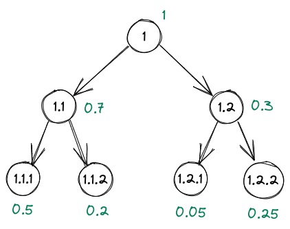
For example, consider the tree in Figure 2, with 2 layers and 2 children at each layer. At the root node, the stick length is 1. It is then broken into two pieces, of length 0.7 and 0.3 respectively. Each of these pieces is then broken down further until we reach the leaves of the tree. Because we can keep breaking the stick, the tree can be arbitrarily wide and deep.

Doubly Recurrent Neural Networks

As in the ETM, the generative process of the TSNTM begins by sampling the latent representation $\mathbf{z}$ from the prior distribution: $\mathbf{z} \sim \mathcal{N}(\mathbf{0}, \mathbf{I})$.

A Doubly Recurrent Neural Network (DRNN) is used to determine the stick-breaking proportions. After randomly initialising the hidden state of the root node, $\mathbf{h}_{1}$, for each topic $k$ the hidden state $\mathbf{h}_{k}$ is given by:

$$\mathbf{h}_{k} = \mathbf{W}_{h} \cdot \operatorname{tanh}(\mathbf{W}_{p} \cdot \mathbf{h}_{\operatorname{par}(k)} + \mathbf{W}_{s} \cdot \mathbf{h}_{k-1})$$

where $\mathbf{h}_{\operatorname{par}(k)}$ is the hidden state of the parent node, and $\mathbf{h}_{k-1}$ is the hidden state of the immediately preceding sibling node (siblings are ordered based on their initial index).

The proportion of the remaining stick allocated to topic $k$, $\nu_{k}$, is given by:

$$\nu_{k} = \operatorname{sigmoid}(\mathbf{z}^{\mathsf{T}} \mathbf{h}_{k})$$

Then, the probability at node $k$, $\pi_{k}$, is given by:

$$\pi_{k} = \pi_{\operatorname{par}(k)} \nu_{k} \prod_{j=1}^{k-1} (1 - \nu_{j})$$

where $j \in \{1, \dots, k-1\}$ are the preceding siblings of node $k$. These are the values in green in Figure 2. The value at each leaf node is the probability for that path (there is only one path to each leaf node).

Now that we have probabilities over the paths of the tree, we need probabilities over nodes within each path. These are computed using another stick-breaking process. At each level of the tree, the hidden state $\mathbf{g}_{l}$ is given by:

$$\mathbf{g}_{l} = \mathbf{W}_{g} \cdot \operatorname{tanh}(\mathbf{W}_{q} \cdot \mathbf{g}_{l-1})$$

This means that all nodes at the same level of the tree have the same value for $\mathbf{g}_{l}$.

The proportion of the remaining stick allocated to level $l$, $\eta_{l}$ is given by:

$$\eta_{l} = \operatorname{sigmoid}(\mathbf{z}^{\mathsf{T}} \mathbf{g}_{l}) \qquad (2)$$

The probability at level $l$, $\theta_{l}$, is given by:

$$\theta_{l} = \eta_{l} \prod_{j=1}^{l-1} (1 - \eta_{j})$$

Empirically, we sometimes found that the most likely words for children nodes in the tree were semantically unrelated to those of their parents. To address this, in Equation 2 we apply a temperature to soften the sigmoid:

$$\eta_{l} = \operatorname{sigmoid}(\psi \mathbf{z}^{\mathsf{T}} \mathbf{g}_{l})$$

In our experiments, we set $\psi = 0.1$. This makes it more likely that when a child node has non-zero probability mass, then its parents will as well (reducing the chance of children nodes being unrelated to their parents).

Training and Inference

The training objective remains the same as in Equation 1; the only change is how $p(x_{w}=v_{w}|\mathbf{z})$ is specified. This is now given by:

$$p(x_{w}=v_{w}|\mathbf{z}) = \sum_{k} \pi_{k} \theta_{\operatorname{level}(k)} \operatorname{softmax}(\mathbf{U} \cdot \mathbf{t}_{k})_{v_{w}}$$

Updating the Tree Structure

So far, the tree structure has been fixed. However we would like this to be learned based on the data. Specifying the exact structure of the tree as a hyperparameter is much harder than simply specifying a number of topics, like we would do for a flat topic model. If we knew the general structure of the tree beforehand, we likely would not need to model the topics. Therefore practical applications of tree-structured topic models need to be able to learn the structure from data. To do this, two heuristic rules are used for adding and deleting nodes to and from the tree. First, the total probability mass at each node is estimated using a random subset of the training data. At node $k$, this estimate is:

$$p_{k} = \frac{\sum_{d=1}^{D} \pi_{k}^{d} \theta_{\operatorname{level}(k)}^{d} N^{d}}{\sum_{d=1}^{D} N^{d}}$$

where $d = \{1,\dots,D\}$ indexes the randomly chosen subset of documents and $N_{d}$ is the number of words in document $d$. Based on these estimates, after every $I$ iterations:

• If $p_{k}$ is above a threshold, a child is added below node $k$ in order to refine the topic.
• If the cumulative sum $p_{k} + \sum_{j \in \operatorname{des}(k)} p_{j}$ is less than a threshold, then node $k$ and its descendants are deleted.

Results on 20 Newsgroups

We run the TSNTM on the same 20 Newsgroups dataset used for training the ETM above. We initialise the tree to have 2 layers with 3 children at each layer. Below is the final tree structure, the top 10 words learned for each topic, and the number of documents which have each topic as their most likely one:

Figure 3: Most likely words for each topic learned by the TSNTM.

Compared to the flat topic model, the tree-structured approach has clear advantages. The tree is automatically learned from the data, with similar topics being grouped together in different parts of the tree. The higher level topics are at the top of the tree (e.g. uninformative words which appear in lots of documents are at the root), and the more refined/specific topics are at the leaves. This makes for results which are much more informative and easier to interpret than the flat model output in Figure 1.

Example documents and the associated topic assignment probabilities learned by the TSNTM are shown

Example 1

We just received an AppleOne Color Scanner for our lab. However, I am having trouble getting reasonable scanned output when printing a scanned photo on a LaserWriter IIg. I have tried scanning at a higher resolution and the display on the screen appears very nice. However, the printed version is coming out ugly! Is this due to the resolution capabilities of the printer? Or are there tricks involved to get better quality? Or should we be getting something (like PhotoShop) to "pretty up" the image? I will appreciate any suggestions. Thanks in advance, -Kris

Example 2

It's over - the Sabres came back to beat the Bruins in OT 6-5 tonight to sweep the series. A beautiful goal by Brad May (Lafontaine set him up while lying down on the ice) ended it. Fuhr left the game game with an injured shoulder and Lafontaine was banged up as well; however, the Sabres will get a week's rest so injuries should not be a problem. Montreal edged Quebec 3-2 to square their series, which seems to be headed for Game 7. The Habs dominated the first two periods and were unlucky to only have a 2-2 tie after 40 minutes. However, an early goal by Brunet in the 3rd won it. The Islanders won their 3rd OT game of the series on a goal by Ray Ferraro 4-3; the Caps simply collapsed after taking a 3-0 lead in the 2nd. The Isles' all-time playoff OT record is now 28-7.

Example 3

Please tell me where I can get a CD on the Wergo Music label for less than $20.

Documents which clearly fall into a specific topic (e.g. the first one) have a high probability at a leaf node whereas those which don't clearly come under any of the learned topics (e.g. the third one) have a high probability at the root node.

Quantitative Evaluation

Topic models are notoriously difficult to evaluate quantitatively. Nevertheless, the most popular metric for measuring topic coherence is the Normalised Pointwise Mutual Information (NPMI). Taking the top M words for each topic, the NPMI will be high if each pair of words $w_{i}$ and $w_{j}$ have a high joint probability $P(w_{i}, w_{j})$ compared to their marginal probabilities $P(w_{i})$ and $P(w_{j})$:

$$\mathrm{NPMI} = \sum_{j=1}^{M} \sum_{i \neq j} \frac{\log \frac{P(w_{i}, w_{j})}{P(w_{i}) P(w_{j})}}{-\log P(w_{i}, w_{j})}$$

The probabilities are estimated using empirical counts.

	NPMI
ETM	0.193
TSNTM	0.227

These results support the qualitative results that the TSNTM is a more coherent model than the ETM.

Incorporating Transformers

Although the TSNTM produces intuitive and easy to interpret results, the learned model still has weaknesses. For example, in Figure 3 the topics relating to politics and space have been grouped under the same parent node. This may not be unreasonable, but their parent node relates to religion, which arguably isn’t coherent. Another more subtle example is that Topic 1.3 groups together computing topics related to both hardware and software; perhaps these should be separated.

We hypothesise that these issues are because the models trained so far have been based on (non-contextual) GloVe embeddings. This can make it difficult to disambiguate words which have different meanings in different contexts. In the past few years, Transformer-based models have achieved state-of-the-art performance for learning informative, contextual representations of text. We look to incorporate Transformer embeddings into the TSNTM.

We follow the approach of the Combined Topic Model (CTM). Instead of using just the bag-of-words representation as the input to the inference model, we now concatenate together the bag-of-words representation with the mean of the final layer states of a Transformer model. Although this is a simple modification, it should allow the inference model to learn a better posterior approximation. For the Transformer model, we use the all-mpnet-base-v2 variant of Sentence-BERT (SBERT), since it achieves consistently high scores on a number of sentence-level tasks.

We train a model which is otherwise identical to the TSNTM from the previous section, except with the SBERT embeddings added to the inference model. Again, below are the top 10 words learned for each topic, and the number of documents which have each topic as their most likely one:

Figure 4: Most likely words for each topic learned by SBERT+TSNTM.

The TSNTM with the SBERT embeddings appears to address some of the incoherence issues of the GloVe-only model. The religion, politics and encryption topics are now grouped under the same parent topic. But unlike with the GloVe-only model, this parent is now a more generic topic whose top words relate to people expressing opinions. The computer hardware and software topics have now been split up, and space is in its own part of the tree. The NPMI also suggests that the model with the SBERT embeddings is more coherent:

	NPMI
ETM	0.193
TSNTM (GloVe only)	0.227
TSNTM (GloVe + SBERT)	0.234

Summary

We have shown that topic models can be a great way to get a high level understanding of a dataset without having to do any labelling.

• ‘Flat’ topic models are the most commonly used but have weaknesses (e.g. output not easiest to interpret, needing to know the number of topics in advance).
• These weaknesses can be addressed by using a tree-structured model which groups related topics together, and automatically learns the topic structure from the data.
• Modelling results can be further improved by using Transformer embeddings.

If you want to try Re:infer at your company, sign up for a free trial or book a demo.