How Machines Learn to Understand Words: A Guide to Embeddings in NLP

Re:infer's machine learning algorithms are based on pre-trained Transformer models, which learn semantically informative representations of sequences of text, known as embeddings. Over the past few years, Transformer models have achieved state of the art results on the majority of common natural language processing (NLP) tasks.

But how did we get here? What has led to the Transformer being the model of choice for training embeddings? Over the past decade, the biggest improvements in NLP have been due to advances in learning unsupervised pre-trained embeddings of text. In this post, we look at the history of embedding methods, and how they have improved over time.

This post will

• Explain what embeddings are and how they are used in common NLP applications.
• Present a history of popular methods for training embeddings, including traditional methods like word2vec and modern Transformer-based methods such as BERT.
• Discuss the weaknesses of embedding methods, and how they can be addressed.

Background

What is an embedding?

Imagine that we have a large corpus of documents on which we want to perform a task, such as recognising the intent of the speaker. Most modern, state of the art NLP methods use neural network based approaches. These first encode each word as a vector of numbers, known as an embedding. The neural network can then take these embeddings as input in order to perform the given task.

Suppose the corpus contains 10,000 unique words. We could encode each word using a 'one-hot' embedding (i.e. a sparse 10,000-dimensional vector with 0s everywhere except in the single position corresponding to the word, where the value is a 1), e.g.

'a' = [1, 0, 0, ..., 0, 0]
...
'my' = [0, ..., 0, 1, 0, ..., 0]
...
'you' = [0, 0, ..., 0, 0, 1]

However, this approach has some problems:

• Semantically uninformative embeddings
  • With the one-hot encoding approach, all of the embeddings are orthogonal to each other. Ideally, we'd like words which are semantically related to each other to have 'similar' embeddings, but one-hot embeddings do not directly encode similarity information.
• High dimensionality
  • Having a 10,000-dimensional vector for each word means we could quickly run out of memory when using a neural network based approach. In many domains, 10,000 is considered a small vocabulary size—vocabularies are often 5–10 times as big.

As a result, lower-dimensional dense embeddings are more popular. As well as addressing the memory issues of one-hot embeddings, they can also encode the idea that two words are semantically similar. For example, suppose we have 4-dimensional dense embeddings. We may want the embeddings for 'apple' and 'banana' to be similar, e.g.

apple = [3.14, -0.03, -0.26, -2.27]
banana = [2.95, -0.18, -0.11, 0.09]

These both have a large positive value in the first position. We may also want the embeddings for 'apple' and 'microsoft' to be similar, e.g.

apple = [3.14, -0.03, -0.26, -2.27]
microsoft = [-0.12, 0.48, -0.05, -2.63]

These both have a large negative value in the fourth position.

How are embeddings used?

Embeddings which encode semantic information are crucial across all NLP applications. Regardless of how well designed the model which consumes them is, if the embeddings are uninformative then the model won’t be able to extract the necessary signals to make accurate predictions.

Classification

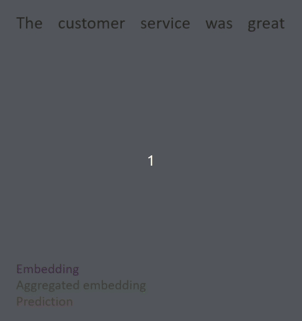
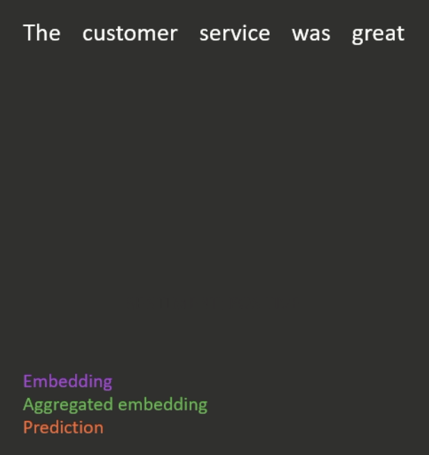
For classification tasks (e.g. sentiment analysis), the most common approach is to aggregate the embeddings for a document into a single vector, and pass this document vector as input into a feedforward network which is responsible for making predictions (see Figure 1 for an illustration).

The aggregate embedding can be computed using a simple heuristic (e.g. taking the mean of the embeddings), or it can itself be the output of a neural network (e.g. an LSTM or Transformer).

Figure 1: Performing sentiment analysis by aggregating the embedding for a document, and using this aggregated embedding to make the prediction.

Semantic search

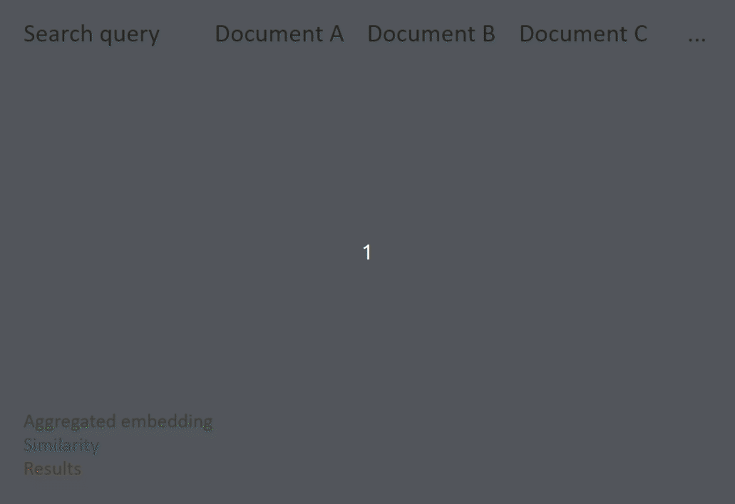
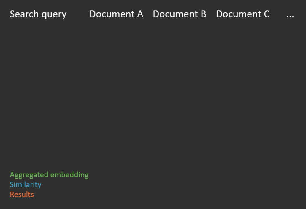
Beyond classification tasks, embeddings are also particularly useful for semantic search. This is the task of retrieving results not only based on keywords, but also based on the semantic meaning of the search query.

Semantic search works by first computing an aggregated embedding for each document in a corpus (again, the aggregation function can be heuristic or learned). Then, the given search query is also embedded, and the documents with the closest embeddings to the embedding of the search query are returned (see Figure 2 for an illustration). Closeness is usually measured according to a metric which compares the distance between two embeddings, for example cosine similarity.

Figure 2: Performing semantic search by comparing the embedding of the search query with each document, and finding the closest match.

A history of embedding methods

Most word embedding methods are trained by taking a large corpus of text, and looking at which words commonly occur next to each other within the sentences in the corpus. For example, the word "computer" may often occur alongside words such as "keyboard", "software", and "internet"; these common neighbouring words are indicative of the information that the embedding of "computer" should encode.

This section covers four popular techniques for learning embeddings, from word2vec to the Transformer based BERT.

word2vec

word2vec, released in 2013, is arguably the first method to have popularised pre-trained word embeddings and brought them into the mainstream in modern NLP. word2vec encompasses two approaches to learning embeddings:

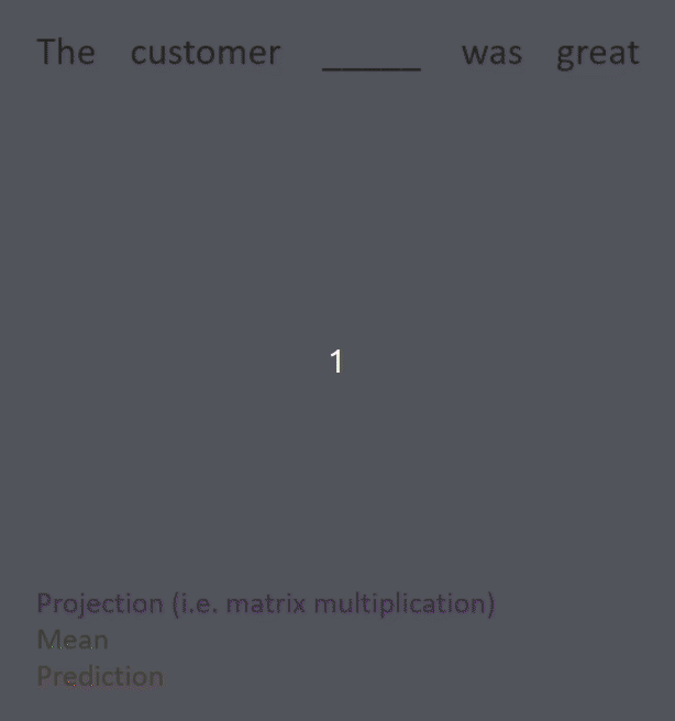
• Continuous bag of words (see Figure 3 for an example).
  • Predict a given word conditioned on the $k$ neighbouring words on either side.
    • This is done by projecting (i.e. matrix-multiplying) the one-hot encodings of the neighbouring words down to lower-dimensional dense embeddings, taking the mean, and using this to predict the missing word.
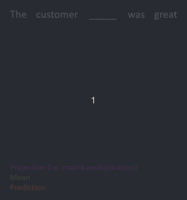
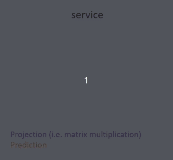
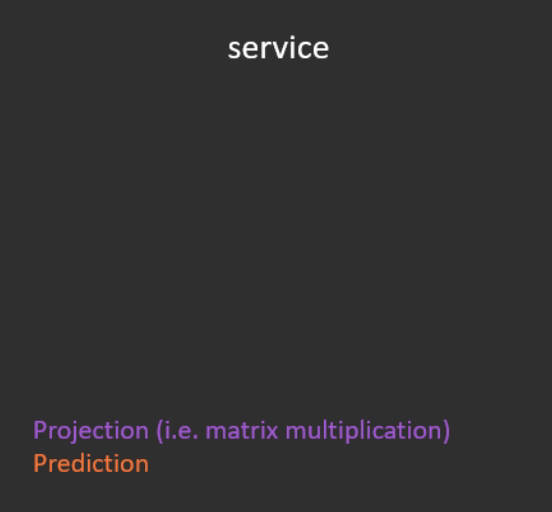
• Skipgram (see Figure 4 for an example).
  • Predict the $k$ neighbouring words on either side given a word.
    • This is done by projecting (i.e. matrix-multiplying) the one-hot encoding of the given word down to a lower-dimensional dense embedding, and using this to predict the missing words.

Figure 3: The word2vec continuous bag of words model.

Figure 4: The word2vec skipgram model.

The authors demonstrate several remarkably intuitive linear analogies between the embeddings. Given two words $x$ and $y$ with a specific relationship, and another word $z$ in the same 'category' as $y$, the authors find the word $w$ whose embedding is nearest (using cosine distance) to $\operatorname{emb}(x) - \operatorname{emb}(y) + \operatorname{emb}(z)$. The resulting word $w$ often has the same relationship to $z$ as $x$ does to $y$ (see Table 1 for some examples).

$x$	$y$	$z$	$w = \operatorname{nearest}(\operatorname{emb}(x) - \operatorname{emb}(y) + \operatorname{emb}(z))$
biggest	big	small	smallest
Paris	France	Italy	Rome
Cu	copper	zinc	Zn

Table 1: Analogies learned by the word2vec model.

GloVe

As described above, word2vec is based on a local sliding window. This means that word2vec doesn't directly make use of global word co-occurrence statistics, except through the number of training examples created. For example, the embeddings don't directly incorporate the fact that the word "bank" occurs more frequently in the context of the word "money" than "river", other than the fact that "bank" and "money" will appear together in more training examples than "bank" and "river".

Therefore, a year after word2vec, GloVe was released, which combines the advantages of local sliding window based approaches with global (i.e. corpus-level) word co-occurrence counts. It does so by training embeddings such that the global co-occurrence count between two words determines how similar their embeddings are.

First, a global co-occurrence matrix $X$ is built, whose entries $X_{i,j}$ indicate how many times word $j$ occurs in the context of word $i$. Then, the GloVe objective trains the word embeddings to minimise the following least squares objective:

$$J = \sum_{i,j \in \mathcal{V}} f(X_{i,j})(\mathbf{u}^{\mathsf{T}}_{i} \mathbf{v}_{j} + b_{i} + c_{j} - \operatorname{log} X_{i,j})^{2}$$

where $\mathcal{V}$ is the vocabulary, $\mathbf{u}$ are word vectors, $\mathbf{v}$ are context vectors, and $b$ and $c$ are biases. $f(X_{i,j})$ is a weighting function to prevent giving too much weight to co-occurrences both with extremely low and extremely high values. Once trained, the final word embedding for word $i$ is $w_{i} = \mathbf{u}_{i} + \mathbf{v}_{i}$.

GloVe embeddings significantly outperform word2vec on the word analogies task (described above), and are slightly better for named entity recognition. As a result, GloVe vectors were the go-to pre-trained word embeddings for a number of years, and still remain popular to date.

info

A key weakness of the methods presented so far is that they are static, i.e. the embedding for a given word is always the same. For example, consider the word "bank"—this may refer to the edge of a river or to a financial institution; its embedding would have to encode both meanings.

To address this weakness, contextual embedding methods were developed. These have a different embedding for each word depending on the sequence (e.g. sentence, document) in which it occurs. This line of work has been game-changing; it is now extremely rare to find state of the art methods which do not rely on contextual embeddings.

ELMo

In the mid-2010s, recurrent neural networks (RNNs) were the most popular architectures for the majority of NLP tasks. RNNs perform computations over sequences of text in a step-by-step manner, reading and processing each word one at a time. They update a 'hidden state', which keeps track of the entire sequence so far.

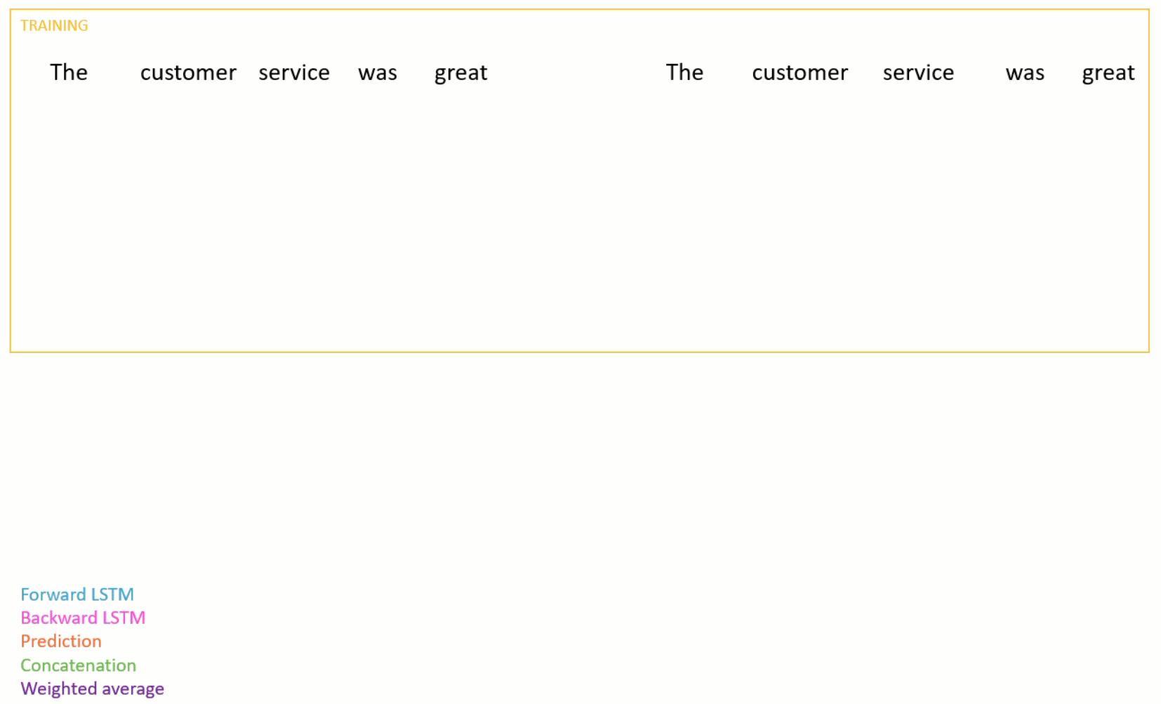
One of the first popular contextual embedding techniques was ELMo, released in 2018. ELMo learns embeddings by pre-training a bidirectional RNN model on a large natural language corpus using a next word prediction objective. Specifically, ELMo trains both a forward and backward stacked LSTM by, at each step, predicting either the next or previous word respectively, as shown in Figure 5.

Once trained, the forward and backward LSTMs' weights are frozen and the outputs are concatenated at each step of each layer. The authors find that the different layers learn different aspects of language—the initial layers model aspects of syntax while the later layers capture context-dependent aspects of word meaning. Therefore a task-specific weighted average over the layers is taken as the embedding for each word.

Figure 5: ELMo, shown with a two-layer bidirectional LSTM.

At the time, ELMo significantly outperformed the previous state of the art methods across a number of tasks, including question answering, recognising textual entailment and sentiment analysis.

BERT

At a similar time to the development of ELMo, the (now famous) Transformer was released as an architecture for performing machine translation. It replaces the sequential computations of RNNs with an 'attention mechanism'—this computes a contextual representation of every word in parallel, and is therefore much faster to run than an RNN.

It was quickly realised that the Transformer architecture could be generalised beyond machine translation to other tasks, including learning embeddings. BERT, released in 2019, is one of the first, and arguably most popular, contextual embedding methods to be based on the Transformer architecture.

However, unlike the methods presented so far, BERT does not directly learn embeddings of words. Instead, it learns embeddings of 'sub-word' tokens. The main problem when learning embeddings of words is that a vocabulary of a fixed size is required—otherwise, we'd run out of memory. Instead, BERT uses an algorithm known as WordPiece to tokenise sentences into sub-word units. This means that words may be split up into separate tokens, e.g. the words {'wait', 'waiting', 'waiter'} may be tokenised as {['wait'], ['wait', '##ing'], ['wait', '##er']}, all sharing the same stem but with different suffixes.

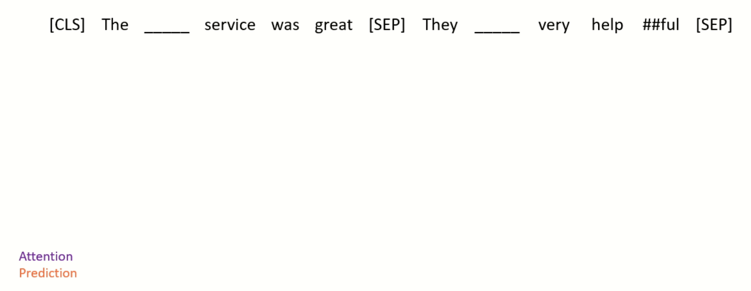
BERT is pre-trained using two objective functions (shown in Figure 6):

• Masked language modelling
  • Some randomly chosen tokens are removed from the sequence, and the model is tasked with predicting them.
• Next sentence prediction
  • Two (masked) sequences are concatenated, with a special [CLS] token at the beginning, and a [SEP] token at the end of each sequence. The model then has to predict whether the second directly follows the first in the original corpus, using the final layer embedding of the [CLS] token.

When performing downstream tasks, the CLS embedding can be used for sentence/document-level tasks e.g. intent recognition or sentiment analysis, while the individual token embeddings can be used for word-level tasks e.g. named entity recognition.

Because the Transformer is not a sequential architecture, the input layer is not simply a projection of the one-hot token encoding. Instead, it is the sum of three different embeddings:

• A projection of the one-hot token encoding.
• A positional embedding (i.e. an embedding of which position the token is in the sequence).
• A segment embedding (i.e. whether the token is from the first sequence or the second, in the next sentence prediction objective described above).

Figure 6: BERT, shown with a one-layer attention mechanism. In reality, all of the attention operations happen at the same time, but here they are shown sequentially for clarity.

Once pre-trained, BERT is usually 'fine-tuned' for downstream tasks (i.e. its weights are further updated for each task; they are not frozen like ELMo). On a number of tasks including SQuAD (question answering) and the GLUE benchmark, BERT significantly outperformed the previous state of the art methods at the time.

BERT (and its follow up variants) have revolutionised the field of NLP; it is now extremely rare to find state of the art methods which do not rely on contextual embeddings based on the Transformer architecture.

Weaknesses of embedding methods

As discussed throughout this post, advances in training embeddings have revolutionised NLP. However, there are certain pitfalls to be aware of when working with pre-trained embeddings.

Firstly, embedding models can encode, and even amplify, the biases contained within the datasets they are trained on. For example, it has been shown that embeddings can encode gender-based occupational stereotypes, e.g. that women are associated with jobs such as homemaking while men are associated with jobs such as computer programming. Further research has shown that embedding models can pick up on derogatory language, racism, and other harmful ideologies from training data. Debiasing language models is an active area of research; the optimal ways to identify and mitigate such biases is still an open question.

Secondly, modern contextual embedding methods involve training models with hundreds of billions of parameters on clusters of thousands of GPUs for several weeks. This can be extremely costly, both financially as well as for the environment. There is a wide range of methods for training more efficient models, as we reviewed previously.

Summary

This post has presented an introduction to the concept of 'embeddings'—dense vectors of numbers which are trained to represent the semantic meaning of sequences of text. This post has

• Explained what embeddings are and how they are used in common NLP applications.
• Presented a history of popular methods for training embeddings, including traditional methods like word2vec and modern Transformer-based methods such as BERT.
• Discussed the weaknesses of embedding methods, and how they can be addressed.