Business runs on communications. Customers reach out when they need something. Colleagues connect to get work done. At Re:infer, our mission is to fundamentally change the economics of service work in the enterprise—to unlock the value in every interaction and make service efficient and scalable. We do this by democratising access to state of the art NLP and NLU.
Specifically, Re:infer models use deep learning architectures called Transformers. Transformers facilitate huge improvements in NLU performance. However, they are also highly compute intensive—both in training the models to learn new concepts and using them to make predictions. This two part series will look at multiple techniques to increase the speed and reduce the compute cost of using these large Transformer architectures.
This post will:
- Present a brief history of embedding models in NLP.
- Explain why the Transformer’s self-attention mechanism has a high computational workload.
- Review modifications to the traditional Transformer architecture that are more computationally efficient to train and run without significantly compromising performance.
The next post, will look at additional computational and approximation techniques that yield further efficiency gains. The next post will:
- Explore distillation techniques, where smaller models are trained to approximate the performance of larger models.
- Explain efficient fine tuning techniques, where parameter updates are restricted.
- Provide our recommendations for when to use each of these methods.
Background
Over the past decade, NLP methods have become significantly better at performing a wide variety of tasks. This can largely be attributed to a shift away from hand-guided, feature-engineering based approaches towards methods driven by machine learning. The biggest improvements in performance have been due to advances in unsupervised pre-trained semantic representation learning. This involves training a model which maps natural language sequences (e.g. words, sentences) to vectors (sequences of numbers) which represent their semantic meaning. These vectors can then be used to perform the task of interest e.g. intent recognition, sentiment classification, named entity recognition, etc.
Word embeddings
The paradigm shift began in the 2010s with word embedding methods such as word2vec and GloVe. These techniques use large natural language datasets to learn embeddings (another word for vectors) of words in an unsupervised manner. The embeddings encode semantic information based on the contexts in which the words frequently occur. For example, the word “computer” may often occur alongside words such as “keyboard”, “software”, and “internet”; these common neighbouring words embody the information that the embedding of “computer” should encode.
Traditional word embeddings have a key weakness—they are static, i.e. the embedding for a given word is always the same. For example, consider the word “bank”—this may refer to the edge of a river or to a financial institution; its embedding would have to encode both meanings.
Contextual embeddings
To address this weakness, contextual embedding methods were developed. These have a different embedding for each word depending on the sequence (e.g. sentence, document) in which it occurs. This line of work has been game-changing; it is now extremely rare to find state of the art methods which do not rely on contextual embeddings.
One of the first popular contextual embedding techniques was ELMo, which involves pre-training a recurrent neural network (RNN) model on a large natural language corpus using a next word prediction objective. The internal representations of this model are then used as the inputs to (typically small) models for performing supervised tasks. At the time, this approach significantly improved on the previous state of the art across several tasks.
RNNs process each word in a sequence one after the other, therefore they can be slow when dealing with long documents. As a result, models like BERT and RoBERTa, which replace the recurrent component of ELMo with the more parallel computation friendly Transformer have become the go-to approaches. These models are usually pre-trained with a masked language modelling objective—a subset of words in a sequence are removed, and the model is tasked to predict what the missing words are.
However, modern Transformer based language models are generally very large—they can contain billions of parameters and are very computationally demanding to run. The typical workflow is:
- Pre-train the language model on a generic unlabelled dataset.
- Further pre-train the language model on a domain-specific unlabelled dataset.
- Fine-tune the language model, using labelled data, to perform the supervised task of interest.
Although the first of these steps is usually a one-off cost, the latter two are not. And whilst computational power is becoming cheaper, Transformer architectures are getting bigger. This means that the cost of state of the art performance isn’t necessarily decreasing.
Therefore this post will present a range of techniques which reduce the computational workload whilst minimising the impact on performance.
The self-attention mechanism
Although Transformers operate on sub-word tokens, this post refers to words throughout in order to keep things easier to understand.
The Transformer architecture begins with a learnable embedding layer. Each subsequent layer builds its internal representations using a ‘self-attention’ mechanism, i.e. the representation for each word looks at every other word in the sequence (see Figure 1 for an example). Each self-attention layer comprises multiple ‘heads’ (each head does its own self-attention).


Suppose there are words in a sequence. Each self-attention head has -dimensional query, key and value vectors for each word, which are computed using the output of the previous layer :
These are concatenated together into the matrices , and respectively. The attention matrix is computed as:
The output of the self-attention layer is then computed as:
The final output for each layer is computed by concatenating the self-attention outputs for each head, and feeding this through a small feedforward network.
Although (unlike RNNs) the computation can be done in parallel, Figure 1 shows that there will be self-attention operations to perform for a sequence with words. That is, the computational complexity scales quadratically with sentence length. When considering that modern Transformers use tens of layers, each with tens of heads consisting of thousands of dimensions, there are lots of operations to perform even for a single sequence.
Naturally, one line of research aims to reduce this complexity with simpler self-attention mechanisms; this is the biggest area of research into efficient Transformer architectures. Some popular approaches are reviewed below; see this survey paper for more comprehensive coverage.
Paying attention block by block
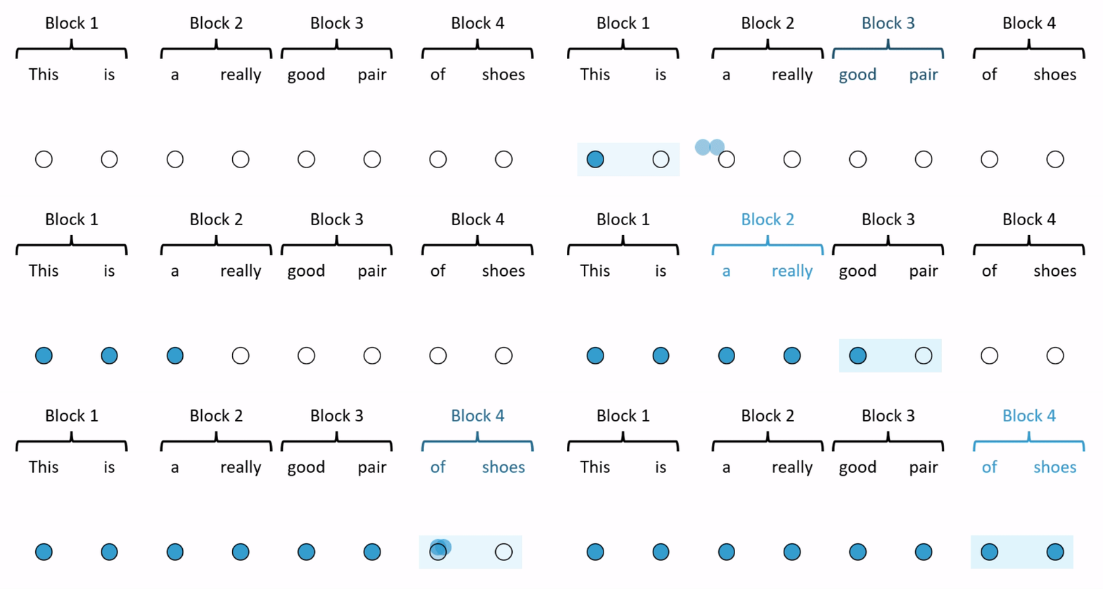
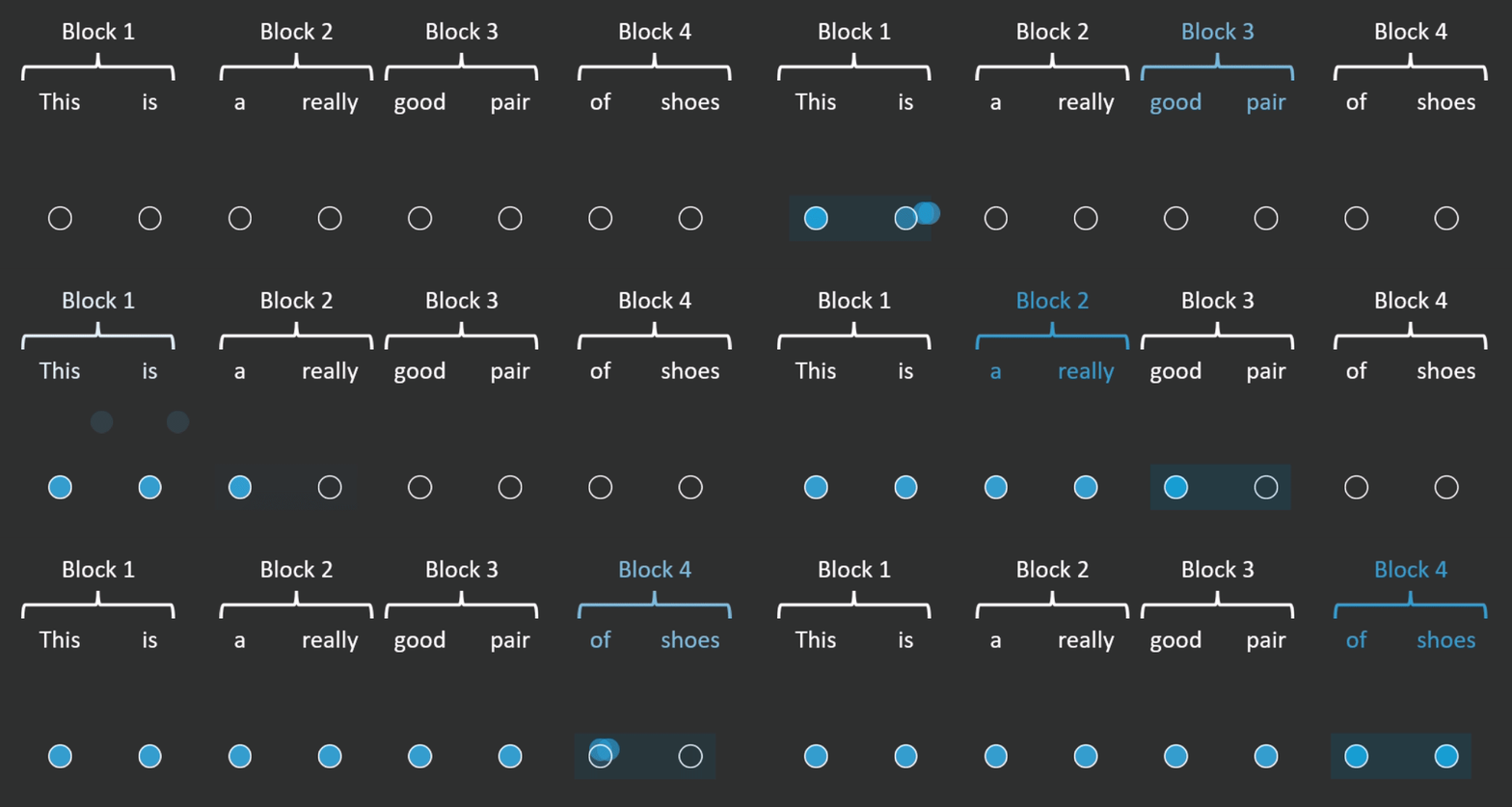
One way to reduce the number of operations is by restricting how many words in the sequence the self-attention mechanism looks at. BlockBERT does this by segmenting the sequence into chunks. At a given attention head, the attention mechanism within a chunk only looks at the words within one of the chunks (see Figure 2 for an example). Every attention head at every layer permutes the chunks that the attention mechanism looks at. This means that after tens of layers, the embedding for each word has likely attended over the entire sequence. Depending on model size, when compared with RoBERTa, BlockBERT is 12%–25% faster to train, requires 19%–36% less memory, and performs almost as well on question answering tasks (F1 scores are ~0.8 points lower on SQuAD 2.0).
Combining multiple attention patterns
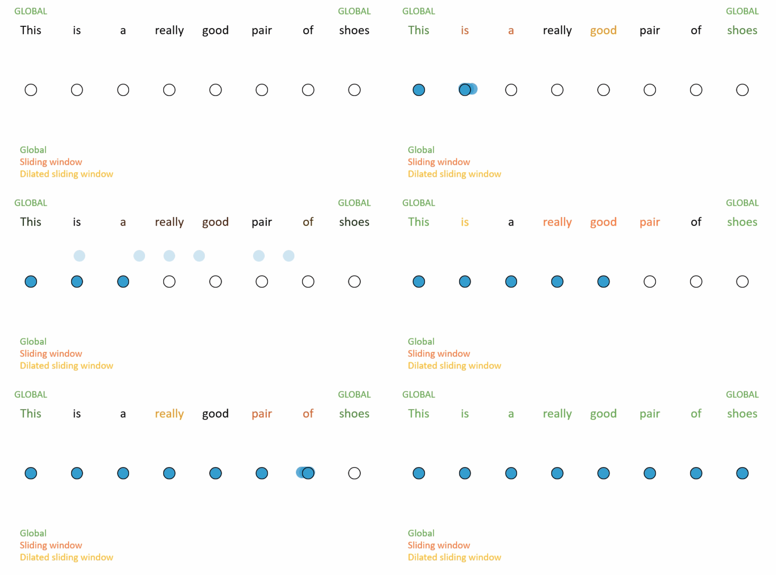
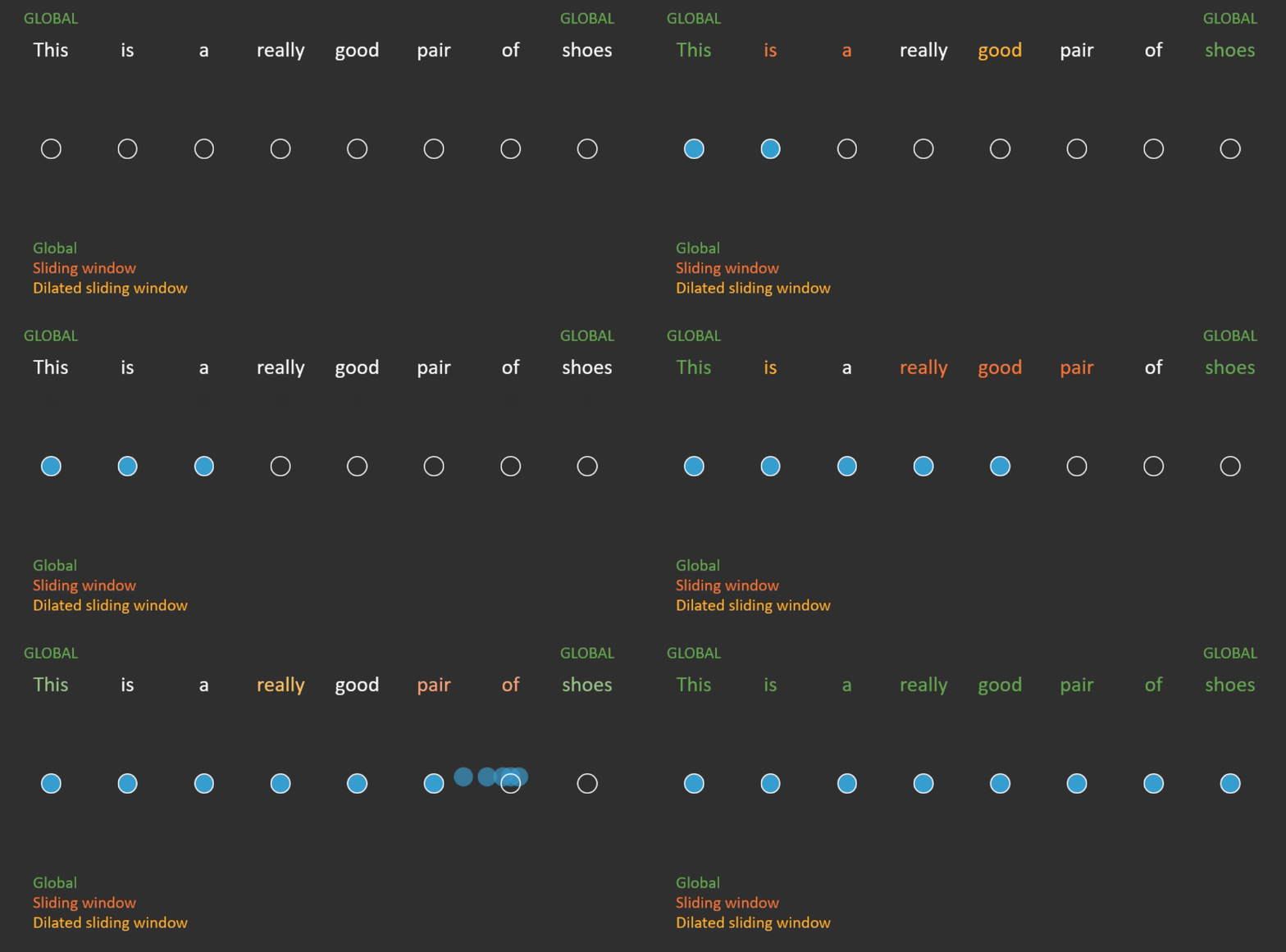
Along similar lines, the Longformer also restricts how many words the self-attention mechanism looks at. It does so by combining multiple simple attention patterns (see Figure 3 for an example).
- Sliding window
- Pay attention only to the neighbouring words.
- Dilated sliding window
- Pay attention to every word, up to a predefined limit.
- Global attention
- At a few pre-selected positions, pay attention to the entire sequence.
- At every position, pay attention to those pre-selected positions.
With this combination of attention patterns, after several layers the embedding for each word has likely attended over the entire sequence. Particularly on long sequences, the Longformer is much faster and uses less memory than RoBERTa. Surprisingly, the Longformer actually outperforms RoBERTa on a variety of tasks—question answering, coreference resolution and sentiment classification.
BigBird is another popular approach and is very similar to the Longformer, except that instead of the dilated sliding window, it uses a random attention pattern (i.e. each representation attends to a fixed number of random words in the sequence).
Using a low rank approximation
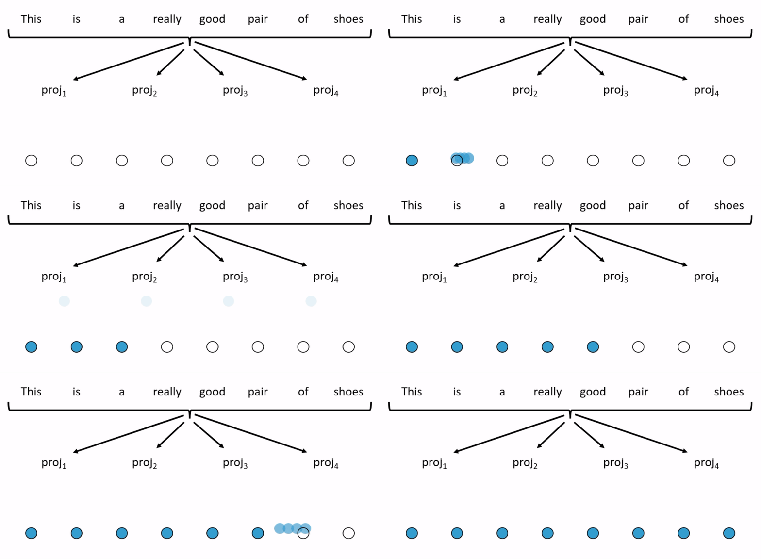
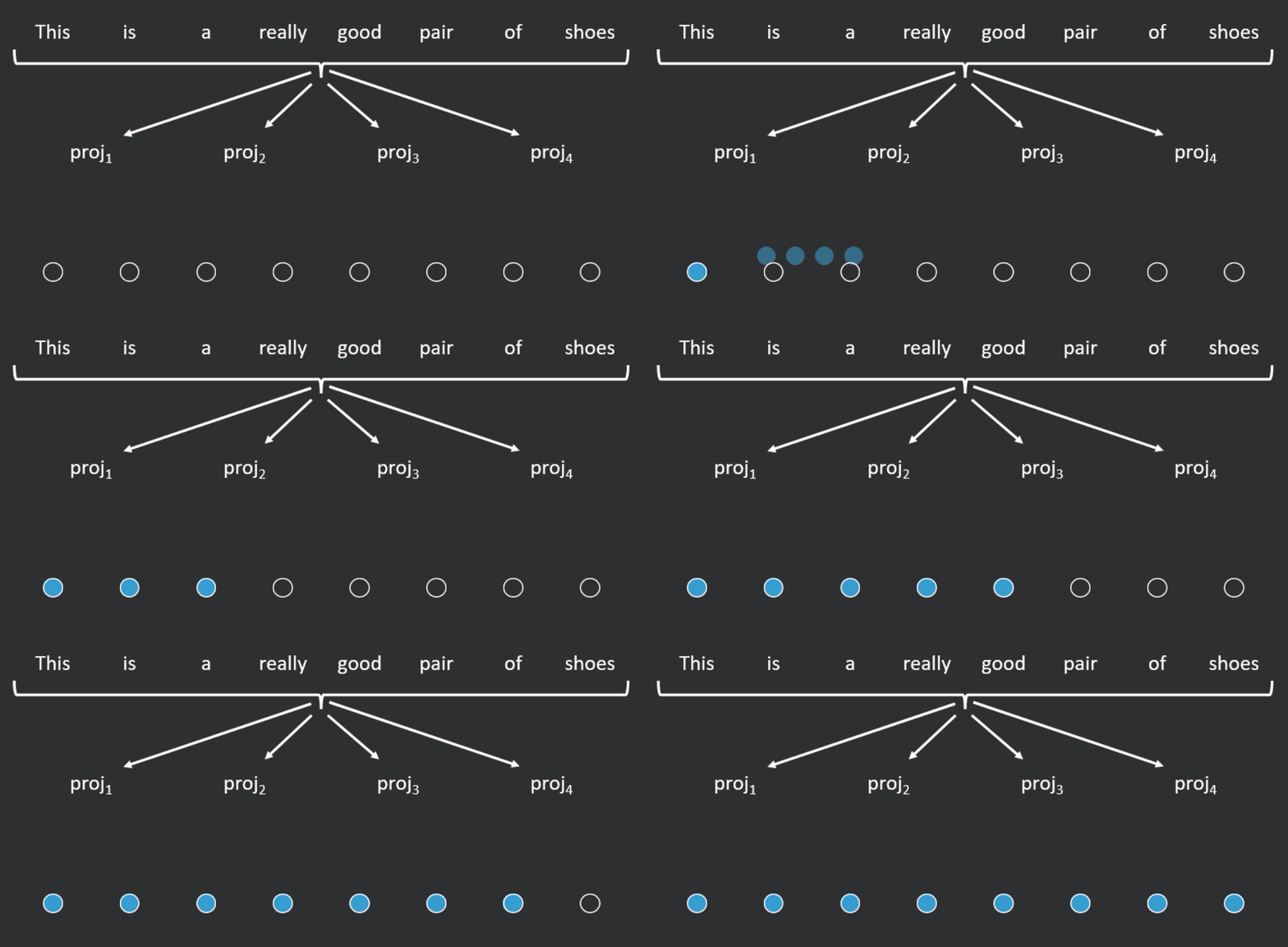
A different type of approach to those presented so far is the Linformer, which is based on the theoretical result that the self-attention operation is low rank. The Linformer linearly projects the key and value matrices ( and ) down, along the length dimension, to a shorter (fixed length) sequence upon which full attention can be applied (see Figure 4 for an example). Compared to standard self-attention, for short sequences, the Linformer is 1.3–3 times faster and for long sequences, it is 3–20 times faster to run. On a variety of text classification tasks, it performs comparably to (and on certain tasks, slightly better than) RoBERTa.
Summary
This two part series looks at how to make state of the art NLP more efficient by exploring modifications to the popular but computationally demanding Transformer-based language modelling techniques. This post:
- Presented a brief history of semantic representation learning in NLP, including traditional word embeddings and contextual embedding models.
- Explained the self-attention mechanism which lies at the heart of the Transformer architecture, and why it is computationally expensive to run.
- Explored alternative attention mechanisms which are more computationally efficient, without sacrificing performance.
The next post will cover:
- An overview of methods which train small models to reproduce the outputs of large models.
- How to fine-tune language models in parameter-efficient ways.
- Our recommendations for scenarios in which to use the different efficient Transformer approaches.
If you want to try Re:infer at your company, sign up for a free trial or book a demo.